
The Visual Representation of High Dimension Spaces
Our brains struggle visualizing spaces with more than 3 dimensions. This is a problem we tried to address in our FaceCloud and FaceField projects. We present here a possible solution using fractional dimensions to represent higher dimensions. The examples here are all based on the Eigenfaces face recognition algorithm where we were dealing with high dimension PCA spaces. But the visualization methodology is not specific to PCA.
The model we used for the Face Field project is a 60-dimensional ‘face space’. That is, we work with 60 Eigenvectors (or Eigenfaces) for all of our operations, be it classic face recognition, the anti-face calculation, or synthetic face generation.
We’ve repeatedly tried to create visualizations of this 60-dimensional space. Working with images makes this easier because one can see immediately what many of the Eigenvectors encode. Working with faces is even better because we’re so tuned to reading faces.
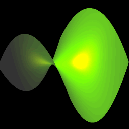
For instance the first Eigenface codes for both lighting and gender.

In this picture we see the ‘mean face’ or ‘average face’ in the center, and the results of shifting the first eigenface’s value (that is, its eigenvalue) from -1 to 1. Note that the face on the left is: female, white face on dark background. The face on the right is: male, dark face on light background.
The coordinates for the mean face are {0,0,0,0,0,…..,0} – zeroes for all 60 eigen values.
The coordinates for the face on the left are {-1,0,0,0,0,…..,0} – minus one for the first eigen value, 0 for the remaining 59.
The coordinates for the face on the right are {1,0,0,0,0,…..,0} – one for the first eigen value, 0 for the remaining 59.
—-
Lets take this a step further and look at the first 3 Eigenfaces. All of the faces below have Eigenvalues of 0 for all Eigenfaces beyond the 3rd one. The values for the first 3 are displayed on the diagram. We have just discussed the first Eigenface in our preceding paragraph. It is represented here by the axis that goes from the upper-left to the lower-right. The second Eigenface seems to encode for side lighting. The third Eigenface encodes for top vs bottom lighting which also incidentally encodes for hair.

But wait, you say, where is the face corresponding to these eigenvalues: {1,1,1}. or {1,1,0} or {-1,0,1}? These are indeed not displayed. One could imagine a cube with the X, Y and Z axes being the first 3 eigen vectors and these other missing faces being the vertices and edges of the cube. So go imagine that because I haven’t got a graphic handy that displays that. Even if I did, what would we have accomplished? Simply displaying 3 dimensions of data in 3 dimensions. The topic of this article concerns High Dimensional Spaces.
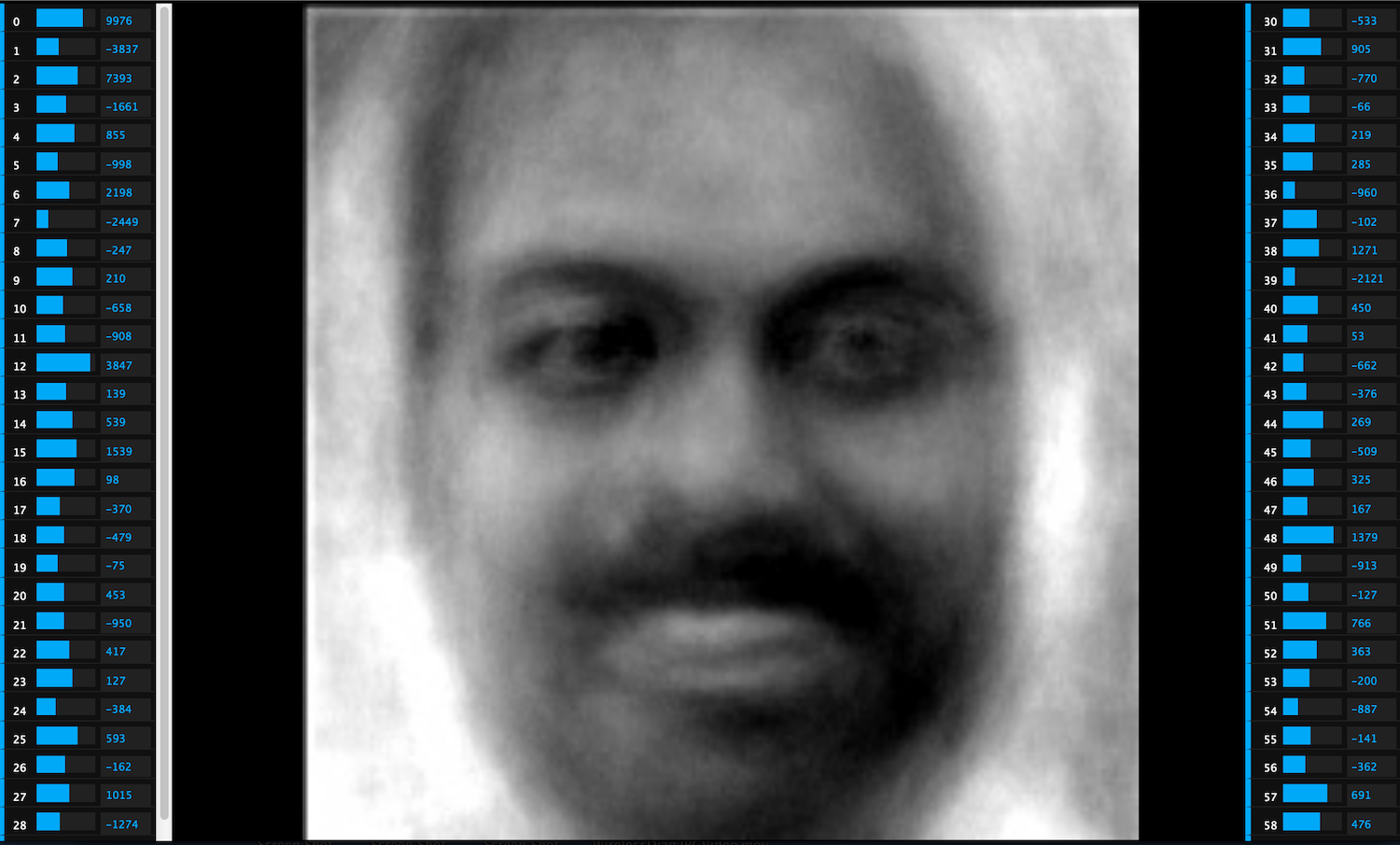
We can take the ‘Face Sextant’ above a step further and use Adelheid Mers’ fractal 3-line matrix to browse a 6 dimensional face space:

I only typed in the coordinates for a few faces. Hopefully you can easily divine what the other values would be. Once again we are missing the edges and vertices of the fractal cube (i.e. the face at {1,1,1,1,1,1} is not on this diagram).
So this process could be repeated over and over-again, adding 3 new dimensions to our visualization on each iteration. It is a loss-less method of representing higher dimensions using smaller and smaller fractal spaces.
In terms of actually making a usable visualization, the faces would get smaller of course so we would need a pan and zoom capability. Here is a visualization using this approach:
Face Cloud from Robert Woodley on Vimeo.
It displays faces with non-zero eigenvalue for the first 12 eigenfaces. In other words it is a visualization of 12 dimensional space. Note also it is using a tetrahedral approach as opposed to a cubic approach. That is, the coordinates for the first 4 faces to emanate from the Mean Face are: {1,1,1}, {-1,-1,1}, {1,1,-1}, {-1,-1,-1}. This reduces the number of faces, thereby reducing the visual clutter and giving the graphics card a chance to keep up with the calculations.
That was a video. The original was written in javascript using three.js and can be run here using chrome on a computer with a good graphics card.
—–
Separately, many of you have seen the Synthetic Face machine. It allows you to tweak all 60 eigen values to get any face you want from the face space, in real-time:
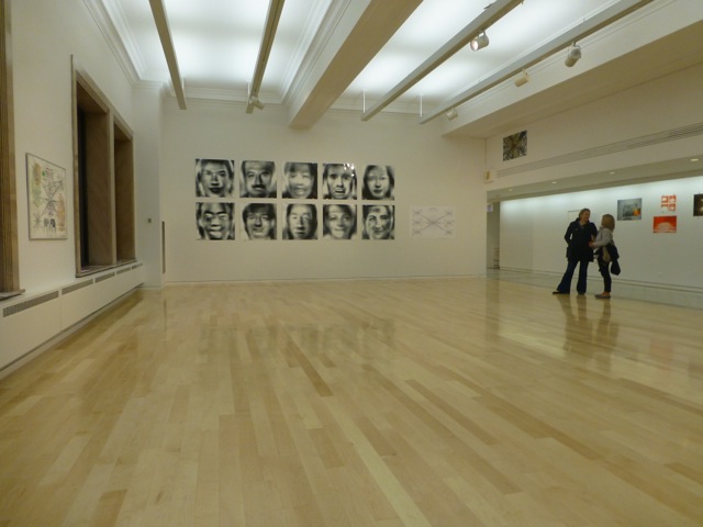
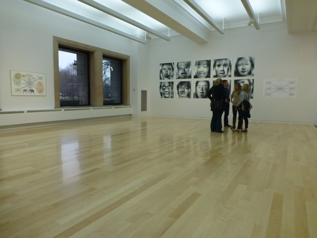
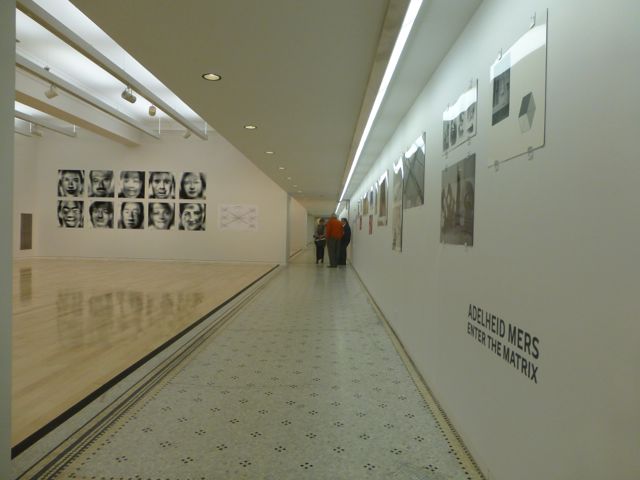
So it is not a way to visualize high dimension spaces, but it is useful for browsing those spaces and pulling faces at random from them. Indeed this was how we generated the faces on display at the “Enter The Matrix” show at the Chicago Cultural Center.
Face Field Update
10 Synthetic Faces are now on display at the Chicago Cultural Center through August, as part of Adelheid Mers’ “Enter the Matrix” exhibit. They look great in large format and are quite powerful. Some photos below.
These are faces pulled at random from the 60-dimensional PCA space that we have been working with for some time now. You can create your own Synthetic Face at http://facefield.org/SynthFace.aspx. (Click on the face that appears for options.)
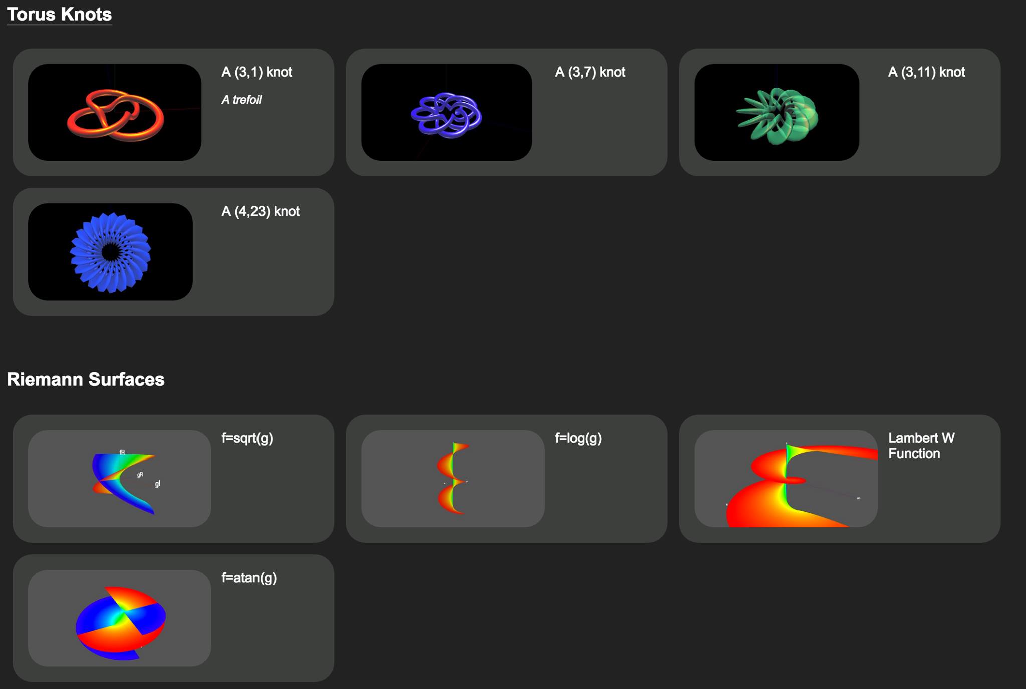
Formula Toy
 Back at the age of 17, thanks to the liberal access policies of Indiana University’s Wrubel Computing Center, I was able to write short little computer programs (on cards!) that would graph 3 dimensional surfaces using a pen plotter. The little nerd that was me was thrilled at the results, and my bedroom wall was plastered with graphs of various mathematical functions of my creation. And incidentally it was an extremely helpful way to get a visual understanding of mathematical geometries, including alternative coordinates systems – cartesian, spherical, and cylindrical.

In these days, there is no shortage of packages that will draw 3-D mathematical surfaces. However, nothing that I found was totally simple. All required a learning curve, or a download or a plugin. I wanted to build something whereby you would simply type in a formula, hit enter, and see the surface. Hence was born Formula Toy. It uses the amazing three.js library which is a wrapper around WebGL. The dependence on WebGL means that it won’t run on every single browser because WebGL is still an emerging standard. However it should work on most MACs and on most Window’s desktops, at least if you use a modern browser like Chrome.
You can either go directly to http://formulatoy.net or you can look at some examples and just click on ones there that intrigue you which will pop you straight into formula toy. There is some help text here.
The Hairy Blob, 800 Ping Pong Balls, and a Mindstorms RoboCam
The Hairy Blob:
At the Hairy Blob exhibition at the Hyde Park Art Center last spring, visitors were invited to draw an image of time on a ping pong ball and toss it into a net that was suspended from the ceiling.


800 Ping Pong Balls:
What to do with over 800 ping pong balls?

How to document 800 three dimensional objects in less than 5 years?
Mindstorms RoboCam:
Our ping pong cam was an NXT Mindstorms robot (which rotated the balls) driven by a laptop that was simultaneously taking pictures. Controlling the robot from an external device was suprisingly difficult. NHK.MindSqualls did the job, but just.
Ping Pong Robo Cam and Laptop setup:


We did the scanning over Thanksgiving weekend at the Roger Brown house in New Buffalo, MI.


The installation:
Intalled at the Mers Micro Museum, a Raspberry Pi drives the display. Some javascript randomly selects from the 800, and then starts a few of them spinning. First it shows a random batch of the day time balls and then a random batch of the night time balls. And so on, indefinitely.


You can also spin the balls online.
Anti-Face Model Specification and Calculation Details
Update 10/2013: We have implemented this in a free iPhone app which is available here:
https://itunes.apple.com/us/app/anti-face/id690376775
Our site FaceField.org (and now the iPhone app) uses the EigenFaces methodology as implemented in Open CV to calculate a special kind of face that we have labelled an ‘Anti Face’.
Model specification:
– Over 1000 faces were used.
– The faces were all facing the camera straight-on. We used a specially designed Haar classifier to ensure that we excluded faces looking to the side.
– The faces that we fed into the PCA calculation are slightly larger than what the Haar classifier detected so that we didn’t cut off the chins.
– The faces were all subject to histogram equalization.
– The faces were all sized to 200×200 pixels.
– We took the first 60 eigenvectors.
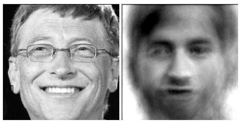
The Antiface calculation is simple: we do a subspace projection of the uploaded face into the 60-dimensional EigenFace space. It is interesting to view this ‘reconstructed face’ as we call it. In a normal face recognition calculation you would then compute the nearest face to this reconstructed face. The anti-face is simply the reconstructed face except that every weight is multiplied by -1.
In other words:
Let Ω ∋ R⁶⁰ be the subspace projection of the uploaded face.
Ω=(w₁,w₂,..w₆₀) where wᵢ= uᵢᵀ(Γ-Ψ) for i=1…60.
u ∋ R⁶⁰ is the Eigenface. Γ is the uploaded face image and Ψ is the mean face.
Then the antiface, Ω’ is (-1*w₁,-1*w₂,..-1*w₆₀).
So prominent features in the reconstructed faces (with high weighting, meaning far from the mean) would be equally prominent, though opposite, in the anti-face.
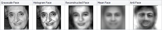
Why 60 dimensions? Originally we tried higher numbers like 200 because at that point the reconstructed face looks indistinguishable from the original face. However the anti-face looks very little like a face and is highly distorted and muddied. It seems that it such high-dimension space not everything looks like a face, however in a lower dimension space like 60 you’re likely to get a face no matter where you land.
Two Face/Anti-Face pairs as examples:

Visualizing Factors and Prime Factorization.
Update 8/2014: The calculator discussed below is also available in the Chrome store here (for free of course).
I’ve previously discussed Brent Yorgey’s factor diagrams. As the father of a 6 year old, I’ve found they are a great way to introduce the concepts of primes and factorization.
Since then, I dabbled with the javascript animations by Sean Seefried to create 2 related products:
1. a calculator, and
2. a factorization game.
Factor Diagram Calculator
The calculator does multiplication and division and allows the young ‘uns to explore the diagrams. I also recently added the ability to do exponentiation after watching Mike Lawler’s video on powers of 3 and Sierpinski’s triangle.
Multiplication:
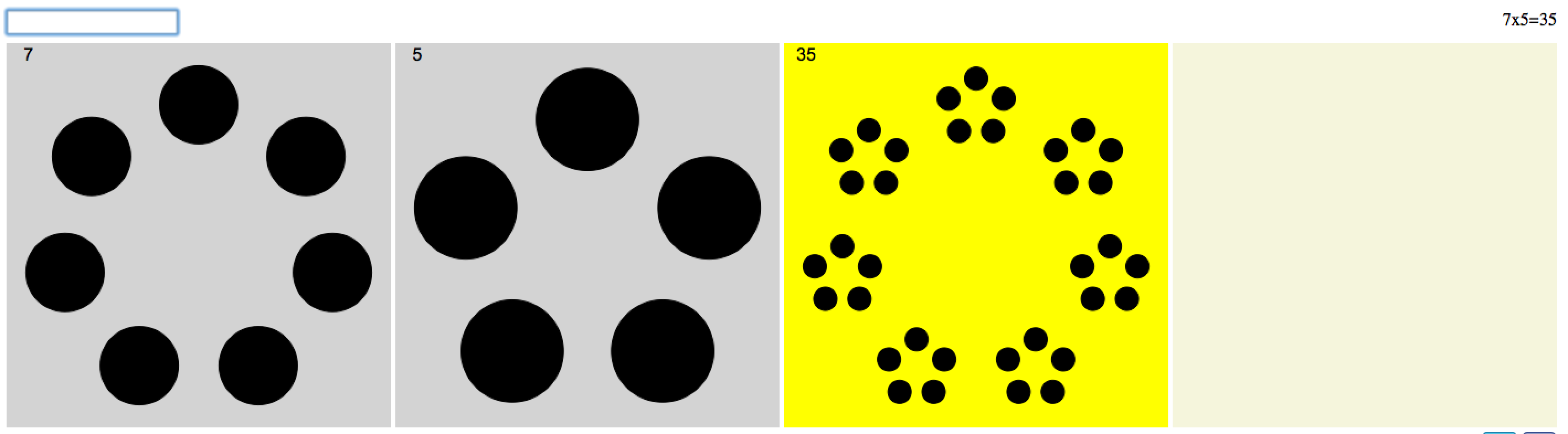
Division:
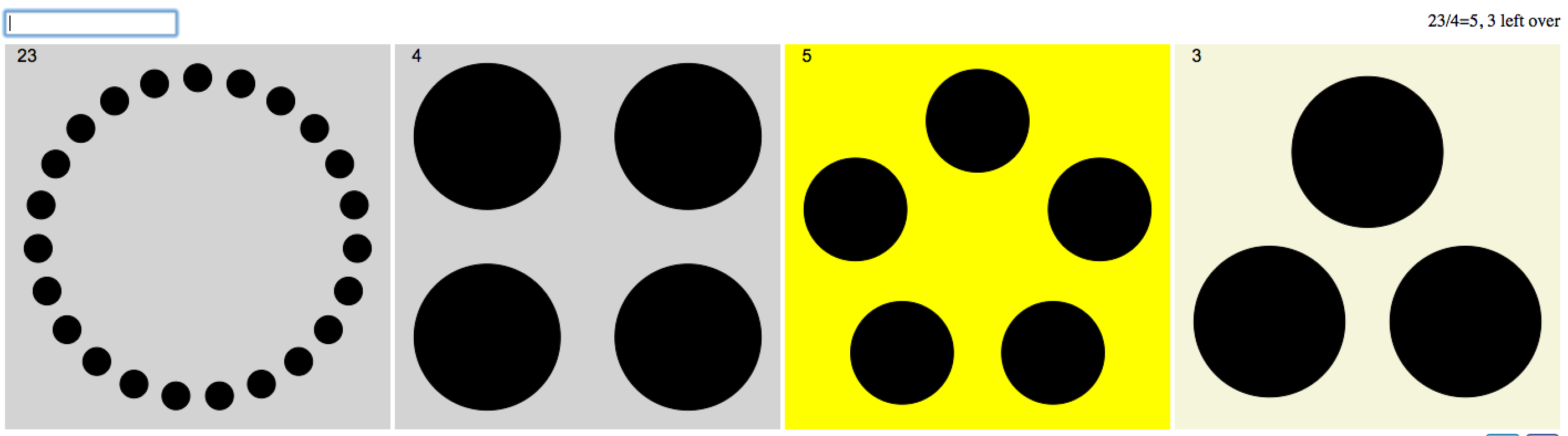
Calculator is here.
Factorization Game
Kids learn by playing, that is well known. So how to make a game out of all of this? I scripted up something simple whereby you’d be presented with a large number and have to factor it while the clock is ticking. Do this a few times, get a score. Then compare with friends collect badges, etc. That last bit (prizes, badges) is not written and is a whole separate app of course.
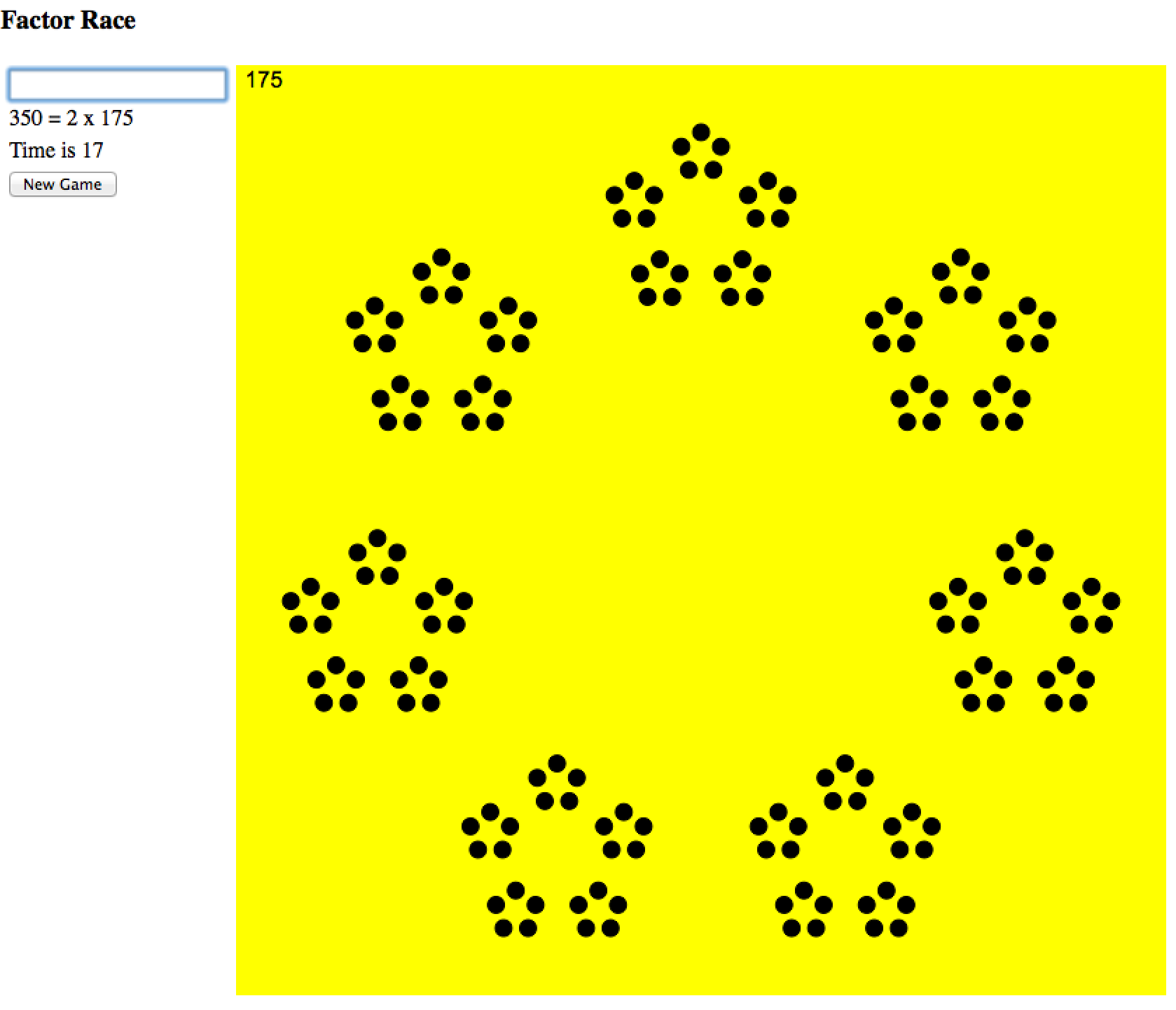
Game is here.
So as it now stands it is simple, a germ of an idea really. Any thoughts on how to improve the learning experience?
Factor Dominoes
Many have discovered Brent Yorgey’s very cool factorization diagrams. They seem like a great way to teach multiplication and factorization to children.
We also were excited by the domino game suggested by Malke Rosenfeld on her blog and decided to try to take her ideas and see if we could create viable game that also would be a fun way to think about factors and primes. To this end we brought together a math geek, a visual artist and a 6 year old ninja and started playing. Through trial and error we arrived at a set of rules.
Simple version of the rules:
Start by printing out a deck of cards. (We have attached a pdf to this post with numbers up to 24 that can be printed on card stock and cut up.)
Each player gets 6 cards. One card is turned face up in the middle. The first player tries to match the turned up card, following the match rules below. After that, players can choose to match the card at either end of the growing chain. If you can’t match then you draw another card. First person to run out of cards wins.
The whole game comes down to the matching rules:
– The number 1 matches anything
– The number 2 matches any even number
– Primes match primes (or as you can explain to a child: circles match circles)
– Other numbers have a major and minor group. For instance 9 has a major group of 3 and a minor group of 3. 15 has a major group of 5 and a minor group of 3. 18 has a major group of 3 and a minor group of 6.
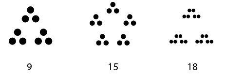
You can match based on major or minor group. If the card you want to play has the same major group or same minor group as the card to be matched, then you can play it. So 10 can match 15 (major group of 5 matches), and 9 can match 15 (minor group of 3 matches). A prime number can match either the minor or the major group, thus 5 can match 10 (major group), but 3 can match 15 (minor group).
Beyond the simple rules:
We started to think about a rule set that might work if you had numbers higher than 24.
Types of number visualizations:
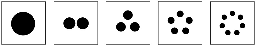
Primes are represented as circles.
Here are the types of Minor Groups:
Simple Minor groups are low primes:
1, 2, 3, 5, 7
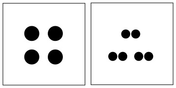
Compounded minor groups:
4 (2×2), 6 (3×2)
Doubly compounded minor groups:
8 (2x2x2), 9 (3x3x3), 16 (4x4x4), 18 (2x3x3)
Triple compounded minor groups:
24 (2x2x2x3), etc.
Major groups
A major group is a combination of N copies of one of these minor or compounded groups.
So here are the generalized matching rules:
– 1 matches anything
– 2 matches any even number
– Minor group types can be matched with each other within types, but not across.
– Major groups can be matched if they have an equal number of elements. For that, minor group types do not have to match.
Attachment:
Here is the pdf you can print out on card stock to make your own set of cards:
Constrain Face Detection for Better Face Recognition
Getting good results with PCA-based facial recognition algorithms depends on correcting for differences in lighting and alignment between the faces. Widely used techniques for correcting for lighting include using histogram equalization or discarding the first eigen vector. Techniques for correcting for alignment differences often involve locating facial features such as the eyes and then rotating the face.
I found these techniques problematic. The corrections for lighting can indeed reduce the impact of overall illumination effects but don’t work for side-lighting scenarios. Face alignment methods are complicated and error prone. In the case of eye alignment one would presumably use additional haar cascades to locate the right eye and the left eye which in turn are error-prone and repeat many of correction problems we have with faces.
It seems that face recognition problems stem from an overly permissive face detection algorithm. The haar cascade that comes with Open CV (called ‘frontalface_alt2’) is indeed very good at detection faces, including rotated faces. It seems it was trained with a sample set that included rotated faces and faces in all different illumination conditions.
Thus constraining face detection so that it only detects horizontal well lit faces would make face recognition much more accurate. That was my hypothesis at any rate and I decided to give it a try.
To this end I used the Open CV tools to build a training set that included only horizontal, full frontal and well lit faces. In the negative sample set I included faces rotated along the Z axis. A better negative set would have included faces rotated along the X and Y axes as well, but I didn’t do that. (By Z axis I mean an axis running vertically through the face).
The resultant cascade is available on https://github.com/rwoodley/iOS-projects/blob/master/FaceDetectionAlgoCompare/OpenCVTest/haarcascade_constrainedFrontalFace.xml. There is a sample iOS application there as well that allows you to compare this cascade with frontalface_alt2 as well as one other cascade.
I was quite pleased with the results. The detection only works on well lit, well aligned faces. This puts the onus on the user to submit a good face. I realize this scenario won’t work with everyone’s system requirements, but in my case it was quite useful.
See the sample output below from my test iPhone application. I aim the camera at a photo of Joe Biden. Above his face are 3 smaller faces in grey-scale. These represent the faces detected by an LBP cascade, the Open CV alt2 cascade and my constrained cascade respectively.

Now see the sample below where Joe Biden’s photo is tilted. The first 2 cascades still find his face, but the 3rd one (the constrained one) does not.

Face Recognition System Design Considerations
Building a face recognition algorithm involves a whole string of design decisions, each of which will impact how well the system can identify faces.
Here is a partial list of these decisions (*):
– Choice of faces used to train the detection algo. Note that both a positive and negative set is needed. In other words you need to show it faces it should recognize, and faces (or other images) it should reject.
– Image preprocessing decisions (size, greyscale, normalization).
– Face alignment corrections.
– Number of eigen vectors to use. In other words, the number of dimensions of your face space.
– Number of low order eigen vectors to exclude. The idea being that low order vectors encode irrelevant (for face recognition) information like lighting.
– Similarity measures. Aka nearest neighbor measures. (Euclidean vs Mahalanobis etc)
– Choice of PCA methodology (Eigenfaces vs Fisherfaces).
After laboriously doing numerous comparisons across multiple training sets on my own, I discovered this paper published in 2001 where some researchers investigated these issues in a very systematic fashion.
Computational and Performance Aspects of PCA-based Face Recognition Algorithms, by H. Moon and P. J. Phillips, Perception, 2001, Vol 30, pg 303-321 and (NISTIR 6486)
http://www.nist.gov/customcf/get_pdf.cfm?pub_id=151458
I was reassured to see that their conclusions were close to my own (which I’ll write up later). It is worth reading the entire paper, but some of main conclusions I took away are:
– Image Normalization helps, but the particular implementation is not critical.
– Performance increases until approximately 200 eigenvectors, then decreases slightly. However much of the performance gain can be captured with 100 eigenvectors.
– Removing the first low-order eigen vectors is best, removing the 2nd helps slightly.
– The similarity measure has a huge effect. Using an enhanced Mahalanobis classifier gives the best result.
(*) note that I’m following the framework implemented in the OpenCV software, namely using Haar classifiers for detection and some form of PCA for recognition.